GSTools: 地统计学工具箱。


项目描述
欢迎使用GSTools


联系方式!


关于GSTools的YouTube教程
目的
GeoStatTools提供各种目的的地统计学工具
- 随机场生成,包括周期性边界
- 简单、普通、通用和外部漂移克里金
- 条件场生成
- 不可压缩随机矢量场生成
- (自动化)变异函数估计和拟合
- 方向变异函数估计和建模
- 数据归一化和转换
- 提供多种现成的甚至用户自定义的协方差模型
- 度量时空建模
- 绘图和导出例程
安装
conda
GSTools可以通过在Linux、Mac和Windows上使用conda进行安装。在命令终端中输入以下命令来安装包
conda install gstools
如果您尚未为您的系统设置conda forge,请参阅conda forge上易于遵循的说明。使用conda,应安装并行化的GSTools版本。
pip
GSTools可以通过Linux、Mac和Windows上的pip进行安装。在Windows上,您可以通过安装WinPython来获取Python和pip运行。在命令终端中输入以下命令来安装包
pip install gstools
要使用pip安装最新开发版本,请参阅文档。需要指出的是,这种方式安装的是GSTools的非并行版本。如果您需要并行版本,请遵循这些简单的步骤。
引用
如果您在出版物中使用GSTools,请引用我们的论文
Müller, S.,Schüler, L.,Zech, A.,和Heße, F.:GSTools v1.3:Python中地质统计学建模的工具箱,Geosci. Model Dev.,15,3161–3182,https://doi.org/10.5194/gmd-15-3161-2022,2022。
您可以通过以下方式引用GSTools的Zenodo代码出版物
Sebastian Müller & Lennart Schüler. GeoStat-Framework/GSTools. Zenodo. https://doi.org/10.5281/zenodo.1313628
如果您想引用特定版本,请查看Zenodo网站。
关于GSTools的文档
您可以在geostat-framework.readthedocs.io下找到文档。
教程和示例
文档还包括一些教程,展示了GSTools最重要的用例,包括
相关的python脚本在examples文件夹中提供。
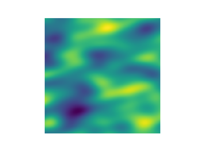
空间随机场生成
这个库的核心是空间随机场的生成。这些场是通过随机化方法生成的,该方法由Heße等人2014年描述。
示例
高斯协方差模型
这是一个使用高斯协方差模型生成二维空间随机场的示例。
import gstools as gs
# structured field with a size 100x100 and a grid-size of 1x1
x = y = range(100)
model = gs.Gaussian(dim=2, var=1, len_scale=10)
srf = gs.SRF(model)
srf((x, y), mesh_type='structured')
srf.plot()
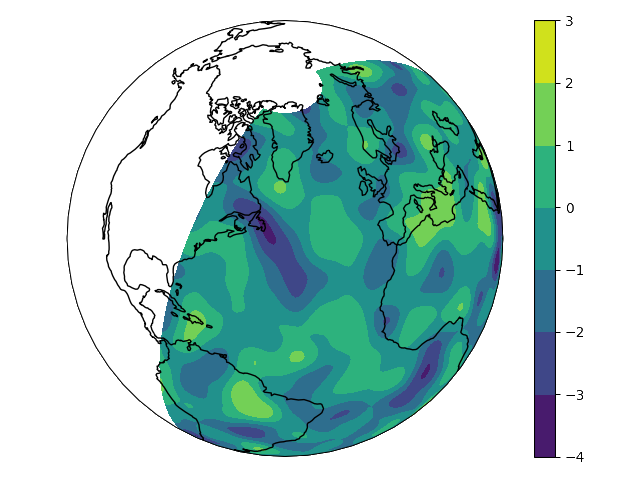
GSTools还支持地理坐标。这可以与cartopy完美配合。
import matplotlib.pyplot as plt
import cartopy.crs as ccrs
import gstools as gs
# define a structured field by latitude and longitude
lat = lon = range(-80, 81)
model = gs.Gaussian(latlon=True, len_scale=777, geo_scale=gs.KM_SCALE)
srf = gs.SRF(model, seed=12345)
field = srf.structured((lat, lon))
# Orthographic plotting with cartopy
ax = plt.subplot(projection=ccrs.Orthographic(-45, 45))
cont = ax.contourf(lon, lat, field, transform=ccrs.PlateCarree())
ax.coastlines()
ax.set_global()
plt.colorbar(cont)
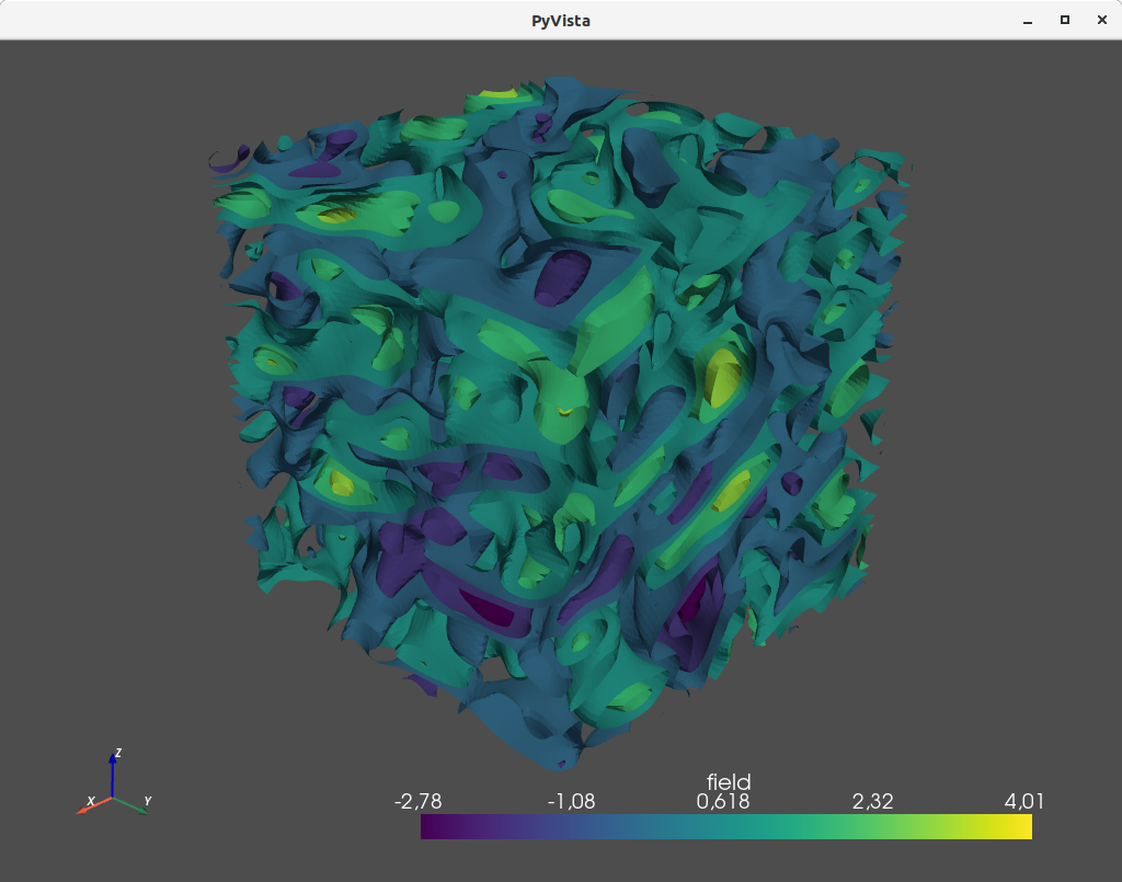
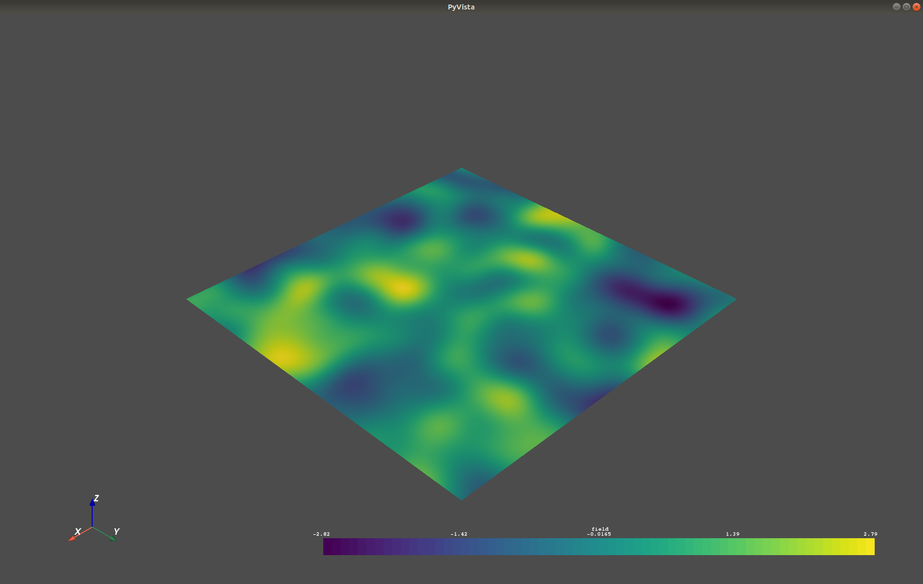
将一个类似的三维场导出到VTK文件中,可以用Python中的ParaView或PyVista进行可视化
import gstools as gs
# structured field with a size 100x100x100 and a grid-size of 1x1x1
x = y = z = range(100)
model = gs.Gaussian(dim=3, len_scale=[16, 8, 4], angles=(0.8, 0.4, 0.2))
srf = gs.SRF(model)
srf((x, y, z), mesh_type='structured')
srf.vtk_export('3d_field') # Save to a VTK file for ParaView

mesh = srf.to_pyvista() # Create a PyVista mesh for plotting in Python
mesh.contour(isosurfaces=8).plot()
估计和拟合变异函数
可以通过变异函数分析场的空间结构,该变异函数包含与协方差函数相同的信息。
所有协方差模型都可以通过简单界面拟合给定的变异函数数据。
示例
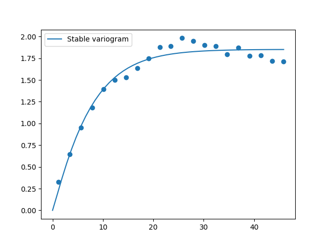
这是一个估计二维无结构场变异函数并再次估计协方差模型参数的示例。
import numpy as np
import gstools as gs
# generate a synthetic field with an exponential model
x = np.random.RandomState(19970221).rand(1000) * 100.
y = np.random.RandomState(20011012).rand(1000) * 100.
model = gs.Exponential(dim=2, var=2, len_scale=8)
srf = gs.SRF(model, mean=0, seed=19970221)
field = srf((x, y))
# estimate the variogram of the field
bin_center, gamma = gs.vario_estimate((x, y), field)
# fit the variogram with a stable model. (no nugget fitted)
fit_model = gs.Stable(dim=2)
fit_model.fit_variogram(bin_center, gamma, nugget=False)
# output
ax = fit_model.plot(x_max=max(bin_center))
ax.scatter(bin_center, gamma)
print(fit_model)
它给出了
Stable(dim=2, var=1.85, len_scale=7.42, nugget=0.0, anis=[1.0], angles=[0.0], alpha=1.09)
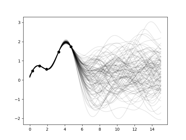
克里金与条件随机场
地统计学的一个重要部分是将克里金与条件空间随机场进行条件化以测量。通过条件随机场,可以生成一系列场实现,其变异性取决于测量的邻近性。
示例
为了更好的可视化,我们将一个一维场条件化到几个“测量”,生成100个实现并绘制它们
import numpy as np
import matplotlib.pyplot as plt
import gstools as gs

# conditions
cond_pos = [0.3, 1.9, 1.1, 3.3, 4.7]
cond_val = [0.47, 0.56, 0.74, 1.47, 1.74]

# conditioned spatial random field class
model = gs.Gaussian(dim=1, var=0.5, len_scale=2)
krige = gs.krige.Ordinary(model, cond_pos, cond_val)
cond_srf = gs.CondSRF(krige)
# same output positions for all ensemble members
grid_pos = np.linspace(0.0, 15.0, 151)
cond_srf.set_pos(grid_pos)

# seeded ensemble generation
seed = gs.random.MasterRNG(20170519)
for i in range(100):
    field = cond_srf(seed=seed(), store=f"field_{i}")
    plt.plot(grid_pos, field, color="k", alpha=0.1)
plt.scatter(cond_pos, cond_val, color="k")
plt.show()
用户定义的协方差模型
gstools的核心特性之一是强大的CovModel类,它允许用户轻松定义协方差模型。
示例
在这里,我们通过定义一个相关函数来重新实现高斯协方差模型,该函数接受一个无量纲距离h = r/l
import numpy as np
import gstools as gs
# use CovModel as the base-class
class Gau(gs.CovModel):
    def cor(self, h):
        return np.exp(-h**2)
这就完成了!现在您有了完整的协方差模型Gau,您可以使用它来生成场或如上所示进行变异函数拟合。
请参阅文档获取有关集成可选参数和优化的更多信息。
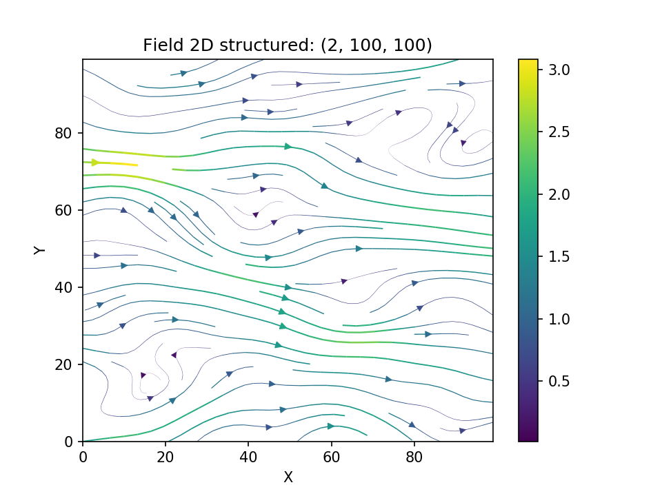
不可压缩矢量场生成
使用原始的Kraichnan方法,可以生成不可压缩的随机空间矢量场。
示例
import numpy as np
import gstools as gs
x = np.arange(100)
y = np.arange(100)
model = gs.Gaussian(dim=2, var=1, len_scale=10)
srf = gs.SRF(model, generator='VectorField', seed=19841203)
srf((x, y), mesh_type='structured')
srf.plot()
产生
VTK/PyVista导出
在创建了一个场之后,您可能希望将其保存到文件中,因此我们提供了一个方便的VTK导出例程,使用.vtk_export(),或者您可以使用.to_pyvista()方法创建一个VTK/PyVista数据集以供Python使用。
import gstools as gs
x = y = range(100)
model = gs.Gaussian(dim=2, var=1, len_scale=10)
srf = gs.SRF(model)
srf((x, y), mesh_type='structured')
srf.vtk_export("field") # Saves to a VTK file
mesh = srf.to_pyvista() # Create a VTK/PyVista dataset in memory
mesh.plot()
这将生成一个RectilinearGrid VTK文件field.vtr或创建一个PyVista网格在内存中,以便在Python中立即进行3D绘图。
要求
可选
联系
您可以通过info@geostat-framework.org联系我们。
许可证
LGPLv3 © 2018-2024


下载文件
下载您平台的文件。如果您不确定选择哪个,请了解有关安装包的更多信息。
源分布
构建版本
gstools-1.6.0.tar.gz 的哈希值
| 算法 | 哈希摘要 | |
|---|---|---|
| SHA256 | df80aad3023427c1390bdbcc004a2dd9e50da6f82c6d849574bb467f098242ce |
|
| MD5 | 9d94103757da650f07912b99af7fe0fd |
|
| BLAKE2b-256 | f1cb804535d50b1376a5bfbef50af5e5cf785525ee03140a19a5daeb8295b596 |
哈希值 为 gstools-1.6.0-cp312-cp312-manylinux_2_17_x86_64.manylinux2014_x86_64.whl
| 算法 | 哈希摘要 | |
|---|---|---|
| SHA256 | 2caaa745d5eeb6d306f7e9be40c52a254b75633607fa202b462083de8514766e |
|
| MD5 | 958fa8594f327c4367b2a8ece4da299b |
|
| BLAKE2b-256 | 4dd4c06ede86c8784c981e79864927ed033f2065af4af084f359bb7ffc569075 |
哈希值 为 gstools-1.6.0-cp312-cp312-macosx_11_0_arm64.whl
| 算法 | 哈希摘要 | |
|---|---|---|
| SHA256 | e5820b078110b6c880fe8f6db09c454c47583be705118a5747677a917b7f82fc |
|
| MD5 | 468033341f33e228c2fb536176064ec1 |
|
| BLAKE2b-256 | 3457fc9e1fb187efc34e6470c5057053ac3b158dda3451940b6894802574229a |
哈希值 为 gstools-1.6.0-cp312-cp312-macosx_10_9_x86_64.whl
| 算法 | 哈希摘要 | |
|---|---|---|
| SHA256 | 8cab1dc2107754a629dd54f951046e5762c4f88950d0a565a67d806b176c5b57 |
|
| MD5 | e37bd88d9b8d2648fdda43517d764023 |
|
| BLAKE2b-256 | c5adbe5f1188c67f1d52fde85b9e98b26a74c2ec6f9ab6a15ea56137f1259c24 |
哈希值 为 gstools-1.6.0-cp311-cp311-manylinux_2_17_x86_64.manylinux2014_x86_64.whl
| 算法 | 哈希摘要 | |
|---|---|---|
| SHA256 | fff329fefb4713268611f021dfaecbda5453d15890073108be57ed638f00c30b |
|
| MD5 | 95923c5249e9dd167331e32ef11f052b |
|
| BLAKE2b-256 | 69a22f93a854cd2292561deb2d2dd7007bd1d1c086aaee9e2130ccdda08e6789 |
哈希值 为 gstools-1.6.0-cp311-cp311-macosx_11_0_arm64.whl
| 算法 | 哈希摘要 | |
|---|---|---|
| SHA256 | 3965a591cec53cf876dfc3777467a767946a980a88aa662c922eac4cb9fa59f1 |
|
| MD5 | 50a1831cf00c21c2cf48b1aaa2ec5df6 |
|
| BLAKE2b-256 | 65626baef59245f0903809e4df4610743a9a3872fb226b7d15076e336181434a |
哈希值 为 gstools-1.6.0-cp311-cp311-macosx_10_9_x86_64.whl
| 算法 | 哈希摘要 | |
|---|---|---|
| SHA256 | ba741e2316e5f5c4e744f556f364d40d29c5c6d2e71246901b032fb7b7f23fef |
|
| MD5 | 4627135ac67fcac3ae81230951a7956e |
|
| BLAKE2b-256 | 88ae9b2a7228f235591b9dcd49eb8bc0a0a7926245e5379536097bee8455c07b |
哈希值 为 gstools-1.6.0-cp310-cp310-manylinux_2_17_x86_64.manylinux2014_x86_64.whl
| 算法 | 哈希摘要 | |
|---|---|---|
| SHA256 | 8748dd8d43c053122de652efb74635327f4a945a537afa0ee2e765e415c72f04 |
|
| MD5 | 0f3418907edf907fcd2e2da925aab813 |
|
| BLAKE2b-256 | 21e8630f616dd3d9cf72688fb81ba842a3a849004aa6e69b8309e17a46806c3e |
哈希值 为 gstools-1.6.0-cp310-cp310-macosx_11_0_arm64.whl
| 算法 | 哈希摘要 | |
|---|---|---|
| SHA256 | 50f3ee9af837ed4a2e08f182f8434219826ab93d94e13f5302c2ff7b5612f4af |
|
| MD5 | 11e98b6d83a2e287c066779fd29a388d |
|
| BLAKE2b-256 | 3f09549247ef74020d9cced146ff646d823da34023cbf8a5895a6eaeddfbe3f9 |
哈希值 为 gstools-1.6.0-cp310-cp310-macosx_10_9_x86_64.whl
| 算法 | 哈希摘要 | |
|---|---|---|
| SHA256 | dd8f8ee9ef90f80076fca480273dc1fecfc832a51a4474b61f0bd1c1e7635872 |
|
| MD5 | 7e807b90fc08445642c72481353dbf31 |
|
| BLAKE2b-256 | 367ef65681e48e9a29f7797961bb86c34a42d8711f90269ba646c1aa66d374a5 |
哈希值 为 gstools-1.6.0-cp39-cp39-manylinux_2_17_x86_64.manylinux2014_x86_64.whl
| 算法 | 哈希摘要 | |
|---|---|---|
| SHA256 | 5942aeaa7c62d5c2b1535dc52f8e71fa8369374c6c94c14d3f8e5de72d1358a1 |
|
| MD5 | 14e4895a2b4c0c01e7bb0df56d189c89 |
|
| BLAKE2b-256 | 7221de17afa92a804a1f26839400a5e13b103d00a49b291ad4d310510c9773f5 |
哈希值 for gstools-1.6.0-cp39-cp39-macosx_11_0_arm64.whl
| 算法 | 哈希摘要 | |
|---|---|---|
| SHA256 | 36b669ec8d198c69577f6230724b88ed9f64ab55b7d0a0cf982fbd8cc3a41ad7 |
|
| MD5 | 81b569cc397f43630ccd685fbfd8b25e |
|
| BLAKE2b-256 | 1512fe73f425a90c4404fb941cb1192235b8626f55271470af0980030215b34c |
哈希值 for gstools-1.6.0-cp39-cp39-macosx_10_9_x86_64.whl
| 算法 | 哈希摘要 | |
|---|---|---|
| SHA256 | 6828fd91a0aa65ef676b4472626f35115d54c86642d1680f5512bdc7f8ec3a97 |
|
| MD5 | 2c30f4517efc7d6fbe89d926f5ca98cb |
|
| BLAKE2b-256 | e2ca7b8478291b26bf49f60838fefdff651fac71b60732113a81c7afa4758891 |
哈希值 for gstools-1.6.0-cp38-cp38-manylinux_2_17_x86_64.manylinux2014_x86_64.whl
| 算法 | 哈希摘要 | |
|---|---|---|
| SHA256 | 67d94769fdb89df53d6e7dd1952a95858c08cf15987f9152d4bf851c19ce6b4a |
|
| MD5 | ec429d89c9a1fa78498af3bd1f224f59 |
|
| BLAKE2b-256 | 06acc45d6346381e980cb5339f29a16f18c516f5df9ba0e555903b7b1e048384 |
哈希值 for gstools-1.6.0-cp38-cp38-macosx_11_0_arm64.whl
| 算法 | 哈希摘要 | |
|---|---|---|
| SHA256 | e45aad48dc4f6c08f40f9832e9d71bb4c4d05e879f7b9d94cd83766c99dc2e40 |
|
| MD5 | aec21384d500b7bc1395d34580840fed |
|
| BLAKE2b-256 | 054fc57fc3749ff89f8d4edb20c4e0ed5d384c13cb215c71089530776d940a59 |
哈希值 for gstools-1.6.0-cp38-cp38-macosx_10_9_x86_64.whl
| 算法 | 哈希摘要 | |
|---|---|---|
| SHA256 | 9125d6a7b1e36a62ca3d9aa7b074722f02e7a7d71934179c09c74bda39a659e7 |
|
| MD5 | 7ee87c546a0d3eaa88f4ab37859730cc |
|
| BLAKE2b-256 | e156e6d1de350f40208bff355794b43053812617801dd4fdb7c7660720a95190 |


