分子化学计算分析和文档的Python API

项目描述
文档: https://pygauss.readthedocs.org
Conda分发: https://binstar.org/cjs14/pygauss
项目: https://github.com/chrisjsewell/PyGauss


PyGauss旨在作为一个交互式工具来支持计算分子化学研究周期的各个阶段,从可视化和分析探索,到文档和发布。
最初PyGauss是为了检查一个或多个Gaussian量子化学计算而设计的,无论是几何上还是电子上。它建立在cclib/chemview/chemlab软件包套件和Python科学堆栈之上,因此应该可以扩展到其他类型的计算化学分析。PyGauss主要设计用于在IPython Notebook中交互式使用。
如示例所示,分子优化可以单独评估(类似于gaussview),也可以作为一组进行。此软件包的优势在于
更快、更有效的分析
可扩展的分析
可重复的分析
快速入门
OSX和Linux
推荐使用Anaconda科学Python发行版(64位)来使用pygauss。下载后,可以在终端中创建一个新环境并安装pygauss
conda create -n pg_env -c https://conda.binstar.org/cjs14 pygauss
Windows
目前没有为Windows或chemlab提供pygauss conda分发,因为chemlab需要使用编译器来构建C扩展。请参阅文档以获取指导。
示例评估
安装 PyGauss 后,您应该可以从以下链接打开此 IPython Notebook: https://github.com/chrisjsewell/PyGauss/blob/master/Example_Assessment.ipynb,然后运行以下操作...
from IPython.display import display, Image
%matplotlib inline
import pygauss as pg
print 'pygauss version: {}'.format(pg.__version__)
pygauss version: 0.6.0
测试文件夹包含多个示例高斯输出,可以进行操作。
folder = pg.get_test_folder()
len(folder.list_files())
33
注意:无论使用本地路径还是通过 ssh(使用 paramiko)的服务器路径,文件夹对象的行为都是相同的。
folder = pg.Folder('/path/to/folder',
                ssh_server='login.server.com',
                ssh_username='username')
单分子分析
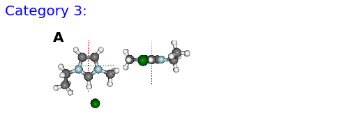
可以创建一个包含初始几何形状、优化过程和最终配置分析的分子。
mol = pg.molecule.Molecule(folder_obj=folder,
                init_fname='CJS1_emim-cl_B_init.com',
                opt_fname=['CJS1_emim-cl_B_6-311+g-d-p-_gd3bj_opt-modredundant_difrz.log',
                           'CJS1_emim-cl_B_6-311+g-d-p-_gd3bj_opt-modredundant_difrz_err.log',
                           'CJS1_emim-cl_B_6-311+g-d-p-_gd3bj_opt-modredundant_unfrz.log'],
                freq_fname='CJS1_emim-cl_B_6-311+g-d-p-_gd3bj_freq_unfrz.log',
                nbo_fname='CJS1_emim-cl_B_6-311+g-d-p-_gd3bj_pop-nbo-full-_unfrz.log',
                atom_groups={'emim':range(20), 'cl':[20]},
                alignto=[3,2,1])
几何分析
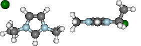
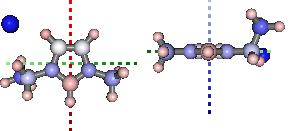
分子可以以静态或交互方式查看。
#mol.show_initial(active=True)
vdw = mol.show_initial(represent='vdw', rotations=[[0,0,90], [-90, 90, 0]])
ball_stick = mol.show_optimisation(represent='ball_stick', rotations=[[0,0,90], [-90, 90, 0]])
display(vdw, ball_stick)
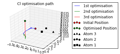
print 'Cl optimised polar coords from aromatic ring : ({0}, {1},{2})'.format(
    *[round(i, 2) for i in mol.calc_polar_coords_from_plane(20,3,2,1)])
ax = mol.plot_opt_trajectory(20, [3,2,1])
ax.set_title('Cl optimisation path')
ax.get_figure().set_size_inches(4, 3)
Cl optimised polar coords from aromatic ring : (0.11, -116.42,-170.06)
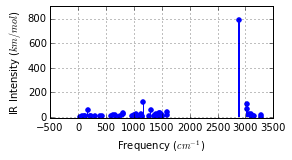
能量和频率分析
print('Optimised? {0}, Conformer? {1}, Energy = {2} a.u.'.format(
    mol.is_optimised(), mol.is_conformer(),
    round(mol.get_opt_energy(units='hartree'),3)))
ax = mol.plot_opt_energy(units='hartree')
ax.get_figure().set_size_inches(3, 2)
ax = mol.plot_freq_analysis()
ax.get_figure().set_size_inches(4, 2)
Optimised? True, Conformer? True, Energy = -805.105 a.u.

几何构象的势能扫描分析...
mol2 = pg.molecule.Molecule(folder_obj=folder, alignto=[3,2,1],
            pes_fname=['CJS_emim_6311_plus_d3_scan.log',
                       'CJS_emim_6311_plus_d3_scan_bck.log'])
ax = mol2.plot_pes_scans([1,4,9,10], rotation=[0,0,90], img_pos='local_maxs', zoom=0.5)
ax.set_title('Ethyl chain rotational conformer analysis')
ax.get_figure().set_size_inches(7, 3)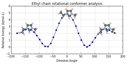
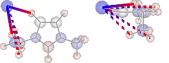
部分电荷分析
使用自然键轨道(NBO)分析
print '+ve charge centre polar coords from aromatic ring: ({0} {1},{2})'.format(
    *[round(i, 2) for i in mol.calc_nbo_charge_center(3, 2, 1)])
display(mol.show_nbo_charges(represent='ball_stick', axis_length=0.4,
                              rotations=[[0,0,90], [-90, 90, 0]]))
+ve charge centre polar coords from aromatic ring: (0.02 -51.77,-33.15)
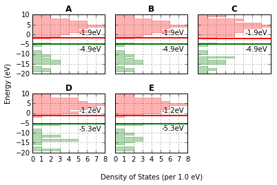
态密度分析
print 'Number of Orbitals: {}'.format(mol.get_orbital_count())
homo, lumo = mol.get_orbital_homo_lumo()
homoe, lumoe = mol.get_orbital_energies([homo, lumo])
print 'HOMO at {} eV'.format(homoe)
print 'LUMO at {} eV'.format(lumoe)
Number of Orbitals: 272 HOMO at -4.91492036773 eV LUMO at -1.85989816817 eV
ax = mol.plot_dos(per_energy=1, lbound=-20, ubound=10, legend_size=12)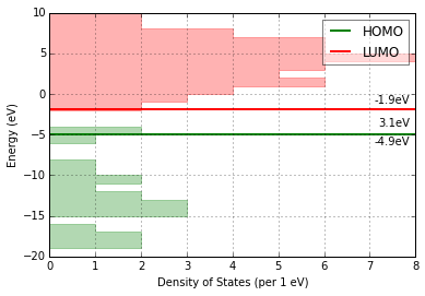
键合分析
使用二阶微扰理论。
print 'H inter-bond energy = {} kJmol-1'.format(
        mol.calc_hbond_energy(eunits='kJmol-1', atom_groups=['emim', 'cl']))
print 'Other inter-bond energy = {} kJmol-1'.format(
    mol.calc_sopt_energy(eunits='kJmol-1', no_hbonds=True, atom_groups=['emim', 'cl']))
display(mol.show_sopt_bonds(min_energy=1, eunits='kJmol-1',
                            atom_groups=['emim', 'cl'],
                            no_hbonds=True,
                            rotations=[[0, 0, 90]]))
display(mol.show_hbond_analysis(cutoff_energy=5.,alpha=0.6,
                                atom_groups=['emim', 'cl'],
                                rotations=[[0, 0, 90], [90, 0, 0]]))
H inter-bond energy = 111.7128 kJmol-1 Other inter-bond energy = 11.00392 kJmol-1

多次计算分析
可以将多个计算(例如不同起始构象的计算)分组到一个 分析 类中,并共同分析。
analysis = pg.Analysis(folder_obj=folder)
errors = analysis.add_runs(headers=['Cation', 'Anion', 'Initial'],
                               values=[['emim'], ['cl'],
                                       ['B', 'BE', 'BM', 'F', 'FE']],
            init_pattern='*{0}-{1}_{2}_init.com',
            opt_pattern='*{0}-{1}_{2}_6-311+g-d-p-_gd3bj_opt*unfrz.log',
            freq_pattern='*{0}-{1}_{2}_6-311+g-d-p-_gd3bj_freq*.log',
            nbo_pattern='*{0}-{1}_{2}_6-311+g-d-p-_gd3bj_pop-nbo-full-*.log',
            alignto=[3,2,1], atom_groups={'emim':range(1,20), 'cl':[20]},
            ipython_print=True)
Reading data 5 of 5
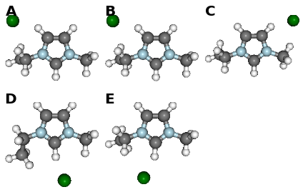
分子比较
fig, caption = analysis.plot_mol_images(mtype='optimised', max_cols=3,
info_columns=['Cation', 'Anion', 'Initial'],
rotations=[[0,0,90]])
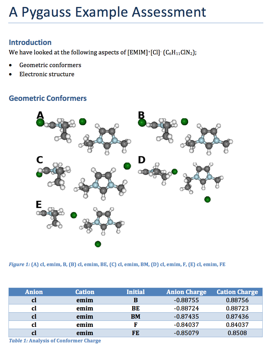
print caption(A) emim, cl, B, (B) emim, cl, BE, (C) emim, cl, BM, (D) emim, cl, F, (E) emim, cl, FE
数据比较
fig, caption = analysis.plot_mol_graphs(gtype='dos', max_cols=3,
lbound=-20, ubound=10, legend_size=0,
band_gap_value=False,
info_columns=['Cation', 'Anion', 'Initial'])
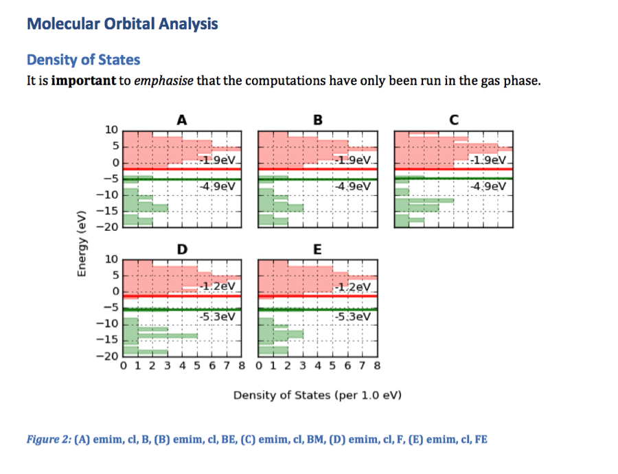
print caption(A) emim, cl, B, (B) emim, cl, BE, (C) emim, cl, BM, (D) emim, cl, F, (E) emim, cl, FE
可以将提到的针对单个分子的方法应用于所有或部分这些计算。
analysis.add_mol_property_subset('Opt', 'is_optimised', rows=[2,3])
analysis.add_mol_property('Energy (au)', 'get_opt_energy', units='hartree')
analysis.add_mol_property('Cation chain, $\\psi$', 'calc_dihedral_angle', [1, 4, 9, 10])
analysis.add_mol_property('Cation Charge', 'calc_nbo_charge', 'emim')
analysis.add_mol_property('Anion Charge', 'calc_nbo_charge', 'cl')
analysis.add_mol_property(['Anion-Cation, $r$', 'Anion-Cation, $\\theta$', 'Anion-Cation, $\\phi$'],
                               'calc_polar_coords_from_plane', 3, 2, 1, 20)
analysis.add_mol_property('Anion-Cation h-bond', 'calc_hbond_energy',
                          eunits='kJmol-1', atom_groups=['emim', 'cl'])
analysis.get_table(row_index=['Anion', 'Cation', 'Initial'],
                   column_index=['Cation', 'Anion', 'Anion-Cation'])
还有选项(需要 pdflatex 和 ghostscript+imagemagik)将表格以 LaTeX 格式图像输出。
analysis.get_table(row_index=['Anion', 'Cation', 'Initial'],
                   column_index=['Cation', 'Anion', 'Anion-Cation'],
                   as_image=True, font_size=12)
多变量分析
RadViz 是一种可视化多变量数据的方法。
ax = analysis.plot_radviz_comparison('Anion', columns=range(4, 10))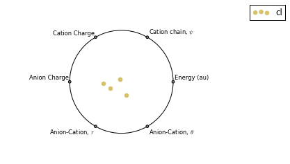
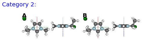
KMeans 算法通过尝试将样本分成具有相同方差的 n 组来聚类数据。
pg.utils.imgplot_kmean_groups(
    analysis, 'Anion', 'cl', 4, range(4, 10),
    output=['Initial'], mtype='optimised',
    rotations=[[0, 0, 90], [-90, 90, 0]],
    axis_length=0.3)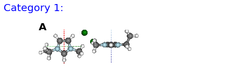
(A) BM
(A) FE
(A) B, (B) BE

(A) F
文档(MS Word)
在分析计算后,您可能想记录一些发现。可以通过通过文件夹对象输出单个图或表图像来实现。
file_path = folder.save_ipyimg(vdw, 'image_of_molecule')
Image(file_path)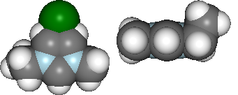
但您可能还想制作一个更完整的分析记录,这时 python-docx 就派上用场了。在此基础上,pygauss MSDocument 类可以生成完整的分析文档。
import matplotlib.pyplot as plt
d = pg.MSDocument()
d.add_heading('A Pygauss Example Assessment', level=0)

d.add_docstring("""
# Introduction

We have looked at the following aspects
of [EMIM]^{+}[Cl]^{-} (C_{6}H_{11}ClN_{2});

- Geometric conformers
- Electronic structure

# Geometric Conformers
""")

fig, caption = analysis.plot_mol_images(max_cols=2,
                rotations=[[90,0,0], [0,0,90]],
                info_columns=['Anion', 'Cation', 'Initial'])
d.add_mpl(fig, dpi=96, height=9, caption=caption)
plt.close()
d.add_paragraph()
df = analysis.get_table(
        columns=['Anion Charge', 'Cation Charge'],
        row_index=['Anion', 'Cation', 'Initial'])
d.add_dataframe(df, incl_indx=True, style='Medium Shading 1 Accent 1',
                caption='Analysis of Conformer Charge')

d.add_docstring("""
# Molecular Orbital Analysis
## Density of States

It is **important** to *emphasise* that the
computations have only been run in the gas phase.
""")
fig, caption = analysis.plot_mol_graphs(gtype='dos', max_cols=3,
                                    lbound=-20, ubound=10, legend_size=0,
                                    band_gap_value=False,
                               info_columns=['Cation', 'Anion', 'Initial'])
d.add_mpl(fig, dpi=96, height=9, caption=caption)
plt.close()

d.save('exmpl_assess.docx')
以下是一些示例
更多内容即将到来!!


pygauss-0.6.0.tar.gz 的哈希值
| 算法 | 哈希摘要 | |
|---|---|---|
| SHA256 | 9e69d46aa6d2b48937ee45b7c7c9ee63a8ab90b606fa1da6aa60429d81728f28 |
|
| MD5 | 3eb9949ee28d88251f9937222afcfc8f |
|
| BLAKE2b-256 | c851a6dadab41f89c0c7808b80c01c855d5a3d70a67f47d9894023ebada3c938 |


