由PyVista提供支持的地图渲染和网格分析


项目描述

基于PyVista的制图渲染和网格分析
| ⚙️ CI |       |
| 💬 社区 |      |
| 📚 文档 |  |
| 📈 健康 |  |
| ✨ 元数据 |     |
| 📦 包 |     |
| 🧰 仓库 |    |
| 🛡️ 状态 |  |
重新发现你的数据
GeoVista建立在巨人的肩膀上,即PyVista和VTK,因此可以轻松利用GPU的强大功能。
因此,它在渲染性能和交互式用户体验方面实现了范式转变,这通过NOAA/NCEP开发的WAVEWATCH III®第三代波浪模型(WAVE高度,WAT水深和
Current Hindcasting)数据实时、时间序列动画得到证明。
动画显示了位于准非结构化球面多细胞(SMC)网格单元面上的海面波显著高度数据的时间序列。
用GeoVista让你的数据生动起来! 🚀
心动了吗?想了解更多?好吧,让我们开始吧...
动机
GeoVista的目标很简单;用便利的制图功能来补充PyVista。
在这方面,从设计角度来看,我们希望尽可能地将GeoVista保持得与PyVista一样纯净,即尽可能减少专业化,以最大限度地提高PyVista和VTK生态系统中的本地兼容性。
我们希望GeoVista成为一个通向PyVista强大世界和它所提供的一切的制图门户。
GeoVista对像geopandas、iris、xarray等这样的包是中立的,这些包专门用于准备你的空间数据以进行可视化。相反,我们将这个责任和工具的选择委托给你,用户,因为我们希望GeoVista尽可能灵活和开放,面向整个科学Python社区。
简单来说,“GeoVista是PyVista”,就像“Cartopy是Matplotlib”一样。好吧,这就是愿望。
安装
GeoVista可在conda-forge和PyPI上获取。
我们推荐使用 conda 来安装 GeoVista 👍
Conda
GeoVista 可在 conda-forge 上找到,并可以使用 conda 简单安装
conda install -c conda-forge geovista
有关更多信息,请参阅我们的 conda-forge 食料 和 prefix.dev 仪表板。
Pip
GeoVista 也可在 PyPI 上找到
pip install geovista
查看我们的 PyPI 下载统计,如果你喜欢这种类型的东西。
快速入门
GeoVista 附带了各种预配置资源,以帮助您开始可视化之旅。
资源
GeoVista 使用各种资源,例如栅格、VTK 网格、自然地球 功能和示例模型数据。
如果您想下载和缓存所有已注册的 GeoVista 资源以使其离线可用,只需
geovista download --all
或者,让 GeoVista 在需要时动态下载资源。
要查看注册资源列表,只需
geovista download --list
想知道更多吗?
geovista download --help
绘图示例
让我们探索使用 GeoVista 的各种海洋学和大气模型数据的样本。
WAVEWATCH III
首先,让我们渲染一个 WAVEWATCH III (WW3) 非结构化 三角网格,使用 10m 自然地球海岸线、一个 1:50m 自然地球交叉混合高程色调 基图层,以及漂亮的感知均匀 cmocean 平衡 分割颜色图。
🗒 点击查看代码
import geovista as gv
from geovista.pantry.data import ww3_global_tri
import geovista.theme

# Load the sample data.
sample = ww3_global_tri()

# Create the mesh from the sample data.
mesh = gv.Transform.from_unstructured(
    sample.lons, sample.lats, connectivity=sample.connectivity, data=sample.data
)

# Plot the mesh.
plotter = gv.GeoPlotter()
sargs = {"title": f"{sample.name} / {sample.units}"}
plotter.add_mesh(mesh, show_edges=True, scalar_bar_args=sargs)
plotter.add_base_layer(texture=gv.natural_earth_hypsometric())
plotter.add_coastlines()
plotter.add_graticule()
plotter.view_xy(negative=True)
plotter.add_axes()
plotter.show()

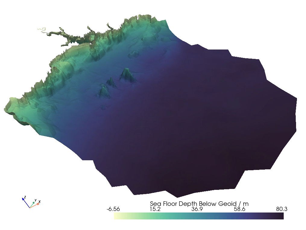
有限体积社区海洋模型
现在,让我们使用由 FVCOM 提供的 非结构化 网格,以及来自 普利茅斯海洋实验室 的丰富 cmocean 深色 颜色图,可视化 普利茅斯 Sound 和 Tamar River 的地形。
🗒 点击查看代码
import geovista as gv
from geovista.pantry.data import fvcom_tamar
import geovista.theme

# Load the sample data.
sample = fvcom_tamar()

# Create the mesh from the sample data.
mesh = gv.Transform.from_unstructured(
    sample.lons,
    sample.lats,
    connectivity=sample.connectivity,
    data=sample.face,
    name="face",
)

# Warp the mesh nodes by the bathymetry.
mesh.point_data["node"] = sample.node
mesh.compute_normals(cell_normals=False, point_normals=True, inplace=True)
mesh.warp_by_scalar(scalars="node", inplace=True, factor=2e-5)

# Plot the mesh.
plotter = gv.GeoPlotter()
sargs = {"title": f"{sample.name} / {sample.units}"}
plotter.add_mesh(mesh, cmap="deep", scalar_bar_args=sargs)
plotter.add_axes()
plotter.show()
CF UGRID
局部区域模型
GeoVista 内部目前支持 圆柱 和 伪圆柱 投影。随着 GeoVista 的成熟和稳定,我们将努力补充其他类别的投影,例如 方位 和 圆锥。
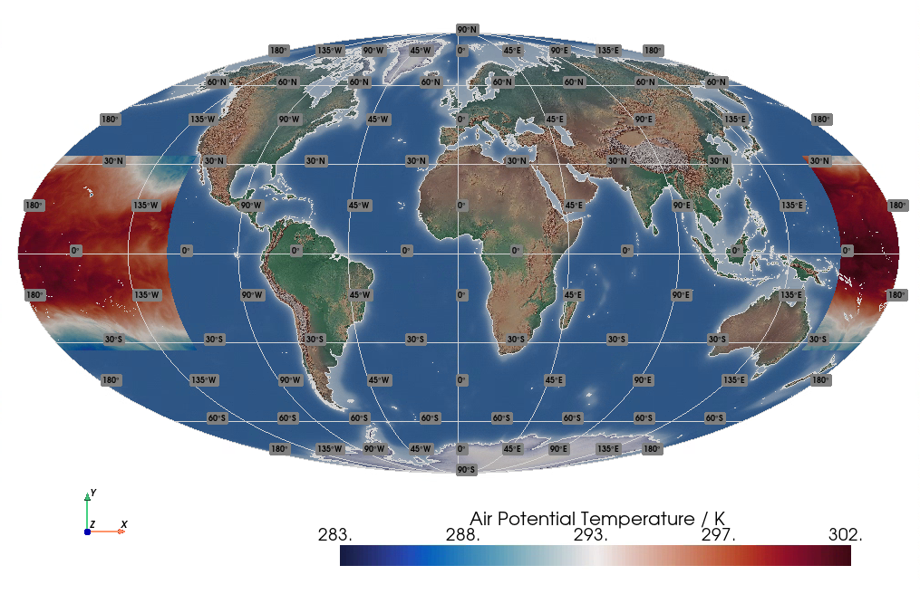
同时,让我们用一些使用 Mollweide 投影并使用 PROJ 字符串重投影的高分辨率 非结构化 局部区域模型 (LAM) 数据来展示我们的基本投影支持,同时使用 10m 自然地球海岸线 和一个 1:50m 自然地球交叉混合高程色调 基图层。
🗒 点击查看代码
import geovista as gv
from geovista.pantry.data import lam_pacific
import geovista.theme

# Load the sample data.
sample = lam_pacific()

# Create the mesh from the sample data.
mesh = gv.Transform.from_unstructured(
    sample.lons,
    sample.lats,
    connectivity=sample.connectivity,
    data=sample.data,
)

# Plot the mesh on a mollweide projection using a Proj string.
plotter = gv.GeoPlotter(crs="+proj=moll")
sargs = {"title": f"{sample.name} / {sample.units}"}
plotter.add_mesh(mesh, scalar_bar_args=sargs)
plotter.add_base_layer(texture=gv.natural_earth_hypsometric())
plotter.add_coastlines()
plotter.add_graticule()
plotter.add_axes()
plotter.view_xy()
plotter.show()
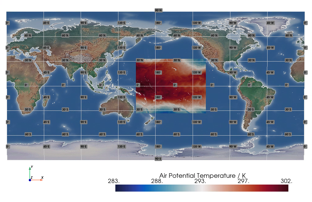
使用相同的 非结构化 LAM 数据,这次使用 等距圆柱 投影,但这次使用 Cartopy Plate Carrée CRS,同样带有 10m 自然地球海岸线 和一个 1:50m 自然地球交叉混合高程色调 基图层。
🗒 点击查看代码
import cartopy.crs as ccrs

import geovista as gv
from geovista.pantry.data import lam_pacific
import geovista.theme

# Load the sample data.
sample = lam_pacific()

# Create the mesh from the sample data.
mesh = gv.Transform.from_unstructured(
    sample.lons,
    sample.lats,
    connectivity=sample.connectivity,
    data=sample.data,
)

# Plot the mesh on a Plate Carrée projection using a cartopy CRS.
plotter = gv.GeoPlotter(crs=ccrs.PlateCarree(central_longitude=180))
sargs = {"title": f"{sample.name} / {sample.units}"}
plotter.add_mesh(mesh, scalar_bar_args=sargs)
plotter.add_base_layer(texture=gv.natural_earth_hypsometric())
plotter.add_coastlines()
plotter.add_graticule()
plotter.add_axes()
plotter.view_xy()
plotter.show()
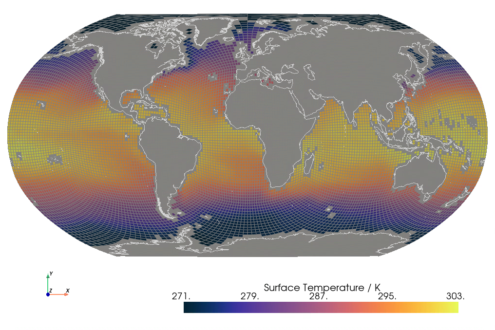
LFRic Cube-Sphere
现在,使用 ESRI SRID 在 Met Office LFRic C48 立方体球体 非结构化 网格上渲染海面温度数据,并使用 Robinson 投影,同时使用 10m 自然地球海岸线 和一个 cmocean 热色 颜色图。
🗒 点击查看代码
import geovista as gv
from geovista.pantry.data import lfric_sst
import geovista.theme

# Load the sample data.
sample = lfric_sst()

# Create the mesh from the sample data.
mesh = gv.Transform.from_unstructured(
    sample.lons,
    sample.lats,
    connectivity=sample.connectivity,
    data=sample.data,
)

# Plot the mesh on a Robinson projection using an ESRI spatial reference identifier.
plotter = gv.GeoPlotter(crs="ESRI:54030")
sargs = {"title": f"{sample.name} / {sample.units}"}
plotter.add_mesh(mesh, cmap="thermal", show_edges=True, scalar_bar_args=sargs)
plotter.add_coastlines()
plotter.view_xy()
plotter.add_axes()
plotter.show()
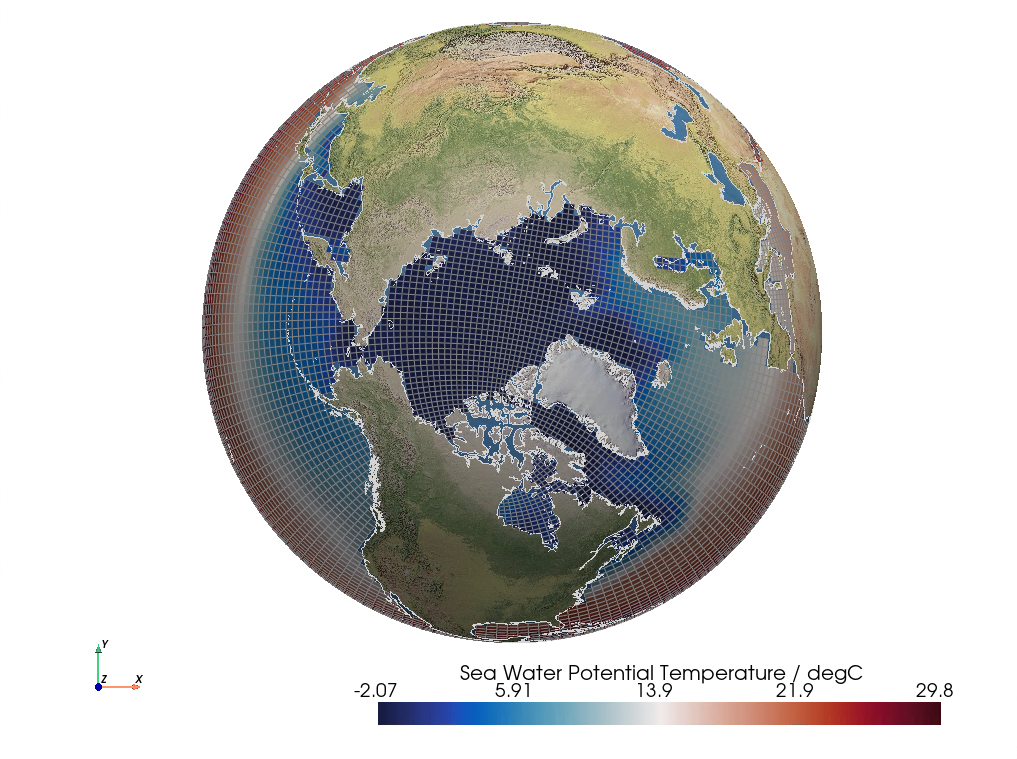
NEMO ORCA2
到目前为止,我们已经展示了GeoVista处理非结构化数据的能力。现在让我们使用欧洲海洋模拟的Nucleus (NEMO) ORCA2海水势温度数据,以及10米自然地球海岸线和1:50米自然地球I基础层,绘制一个曲线网格。
🗒 点击查看代码
import geovista as gv
from geovista.pantry.data import nemo_orca2
import geovista.theme

# Load sample data.
sample = nemo_orca2()

# Create the mesh from the sample data.
mesh = gv.Transform.from_2d(sample.lons, sample.lats, data=sample.data)

# Remove cells from the mesh with NaN values.
mesh = mesh.threshold()

# Plot the mesh.
plotter = gv.GeoPlotter()
sargs = {"title": f"{sample.name} / {sample.units}"}
plotter.add_mesh(mesh, show_edges=True, scalar_bar_args=sargs)
plotter.add_base_layer(texture=gv.natural_earth_1())
plotter.add_coastlines()
plotter.view_xy()
plotter.add_axes()
plotter.show()
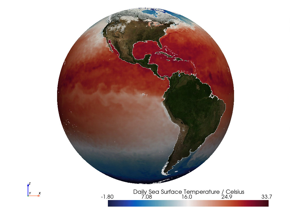
OISST AVHRR
现在让我们渲染一个NOAA/NCEI最优插值海表温度 (OISST) 高分辨率辐射计 (AVHRR) 的矩形网格,使用10米自然地球海岸线和NASA蓝宝石基础层。
🗒 点击查看代码
import geovista as gv
from geovista.pantry.data import oisst_avhrr_sst
import geovista.theme

# Load sample data.
sample = oisst_avhrr_sst()

# Create the mesh from the sample data.
mesh = gv.Transform.from_1d(sample.lons, sample.lats, data=sample.data)

# Remove cells from the mesh with NaN values.
mesh = mesh.threshold()

# Plot the mesh.
plotter = gv.GeoPlotter()
sargs = {"title": f"{sample.name} / {sample.units}"}
plotter.add_mesh(mesh, scalar_bar_args=sargs)
plotter.add_base_layer(texture=gv.blue_marble())
plotter.add_coastlines()
plotter.view_xz()
plotter.add_axes()
plotter.show()
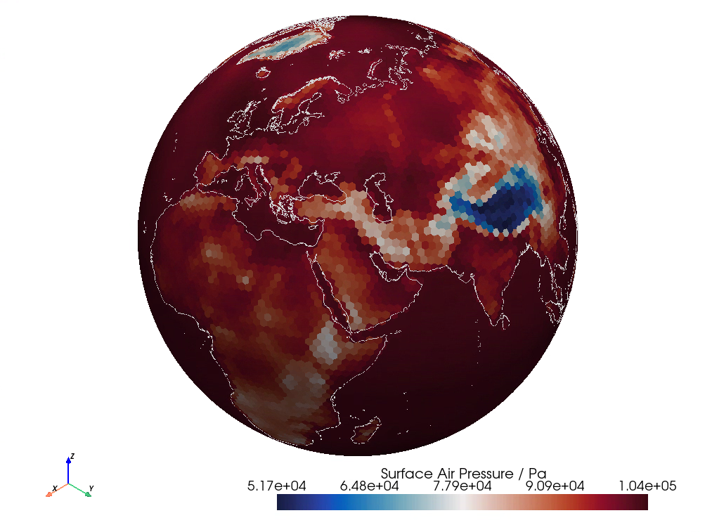
DYNAMICO
最后,为了展示对非传统单元几何形状的支持,例如不是三角形或四边形,我们绘制了来自DYNAMICO项目的非结构化网格。该模型使用六边形和五边形单元,是LMD-Z大气环流模型(GCM)的一部分,是IPSL-CM地球系统模型的新动态核。渲染还包含10米自然地球海岸线。
🗒 点击查看代码
import geovista as gv
from geovista.pantry.data import dynamico
import geovista.theme

# Load sample data.
sample = dynamico()

# Create the mesh from the sample data.
mesh = gv.Transform.from_unstructured(sample.lons, sample.lats, data=sample.data)

# Plot the mesh.
plotter = gv.GeoPlotter()
sargs = {"title": f"{sample.name} / {sample.units}"}
plotter.add_mesh(mesh, scalar_bar_args=sargs)
plotter.add_coastlines()
plotter.add_axes()
plotter.show()
更多示例
"请,先生,我还要一些", 查尔斯·狄更斯,《雾都孤儿》,1838。
当然,我们的荣幸!从命令行,只需
geovista examples --run all --verbose
想知道更多吗?
geovista examples --help
文档
该文档由Sphinx构建,并托管在Read the Docs上。
生态系统
当你在这里时,为什么不访问pyvista-xarray项目并查看它呢!
它旨在为xarray社区提供xarray DataArray访问器,以在3D中可视化数据集,并将建立在GeoVista之上🎉
支持
需要帮助吗?😢
为什么不查看我们现有的GitHub问题。看到类似的问题吗?好吧,给它一个👍来提高其优先级,并随时参与对话。否则,请毫不犹豫地创建一个新的GitHub问题。
然而,如果你更愿意闲聊,那么请访问我们的GitHub讨论。那里绝对是谈论GeoVista的一切的好地方!
许可证
GeoVista是在BSD-3-Clause许可下分发的。
星历史

#ShowYourStripes

图形和首席科学家: Ed Hawkins,英国雷丁大学国家大气科学中心。
数据:伯克利地球,NOAA,英国气象局,瑞士气象局,DWD,SMHI,UoR,法国气象局 & ZAMG。
#ShowYourStripes是在Creative Commons Attribution 4.0 International License下分发的


下载文件
下载适用于您平台上的文件。如果您不确定选择哪个,请了解更多关于安装包的信息。
源代码分发
构建分发
geovista-0.5.2.tar.gz的哈希值
| 算法 | 哈希摘要 | |
|---|---|---|
| SHA256 | c4dcb031cee3af2fae22787b5cae93b3df137eda05ecdd48becfdca3317d021a |
|
| MD5 | 250755a684f72e67568995e20a60759a |
|
| BLAKE2b-256 | 48e557b302810af115214726643f50cf1def055c8d378b3f0e0f06bc42a346f0 |
geovista-0.5.2-py3-none-any.whl的哈希值
| 算法 | 哈希摘要 | |
|---|---|---|
| SHA256 | bcbadfeb70483a6ace85db16d9482b847fe760dde5e3818c41fbc6d7a7557570 |
|
| MD5 | 5a4a169f05a6f39fc86e649d11918fcf |
|
| BLAKE2b-256 | f991e7dc1d0565e69642c4c1f384ffe34f8226717b144056859a4f5bda80a105 |


